Image Mosaicing
RGB Image Mosaicing via Multi-graph synchronization
Image mosaicing is an effective means of constructing a single seamless image by aligning multiple partially overlapped images. Over the years several different approaches have been proposed to solve the various steps of the mosaicing pipeline such as alignment and compositing. My project aims to propose a solution for Global Homography Estimation, a fundamental step of image alignment, based on the multi-graph synchronization algorithm MULTISYNC, Dal Cin et al.
I presented this project with Dr. Francesco Azzoni and Dr. Corrado Fasana to the Computer Vision exam in Politecnico di Milano.
I already analyzed the basic idea behind MULTISYNC approach in this blog post which I suggest you to read before continuing, since I will start from it and I will go more in depth to analyze our project and our experiments.
To summarize, MULTISYNC is based on multi-graph synchronization used for the image alignment step. The whole procedure can be seen as composed of three main steps:
- Graph Building: in this phase, the graph representation of the pairwise homographies, able to align one image to another one, is built.
- Image Alignment: in this phase, multi-graph synchronization is applied to the previously constructed graph. Thanks to the synchronization algorithm, the unknown states representing global homographies are inferred. Differently from pariwise hommographies, global homographies are able to align the images to the common coordinate system.
- Image Stitching: in this phase, the stitched image is created. Each image is transformed in the reference frame by exploiting the estimated global homographies and fused with the others.
In the following, we provide some definitions that are useful for a better understanding of the project.
Multi-graph
A multi-graph \(\mathcal{G} = (\mathcal{V}, \mathcal{E}, s, t)\) is a directed graph with multi-edges, where \(\mathcal{V}\) is the set of vertices, \(\mathcal{E}\) is the set of edges, \(s: \mathcal{E} \to \mathcal{V}\) is a function that maps an edge to its source vertex, and \(t: \mathcal{E} \to \mathcal{V}\) is function mapping an edge to its target vertex.
Multi-edge (Multi-arc)
Considering a multi-graph \(\mathcal{G} = (\mathcal{V}, \mathcal{E}, s, t)\), the multi-edge \(E(i, j)\) is the set of edges having the same source and destination vertices:
\[\begin{gathered} E(i, j) = \{ e \in \mathcal {E} \colon s(e) = i \land t(e) = j \}. \end{gathered}\]Group-labeled multi-graph
A \(\Sigma\)-labeled multi-graph is a tuple \(\Gamma = (\mathcal{V}, \mathcal{E}, s, t, z)\) where \(\mathcal{G} = (\mathcal{V}, \mathcal{E}, s, t)\) is a multi-graph and \(z: \mathcal{E} \to \Sigma\) is the edge labeling function. The edge set \(\mathcal{E}\) satisfies the following property: if \(e \in \mathcal{E}\) with \(s(e) = u \land t(e) = v\), then \(e' \in \mathcal{E}\) with \(s(e') = u \land t(e') = v\), and \(z\) satisfies:
\[z(e) = z(e')^{-1}\]Consistent labeling
Let \(\Gamma = (\mathcal{V}, \mathcal{E}, s, t, z)\) be a \(\Sigma\)-labelled multi-graph and let \(x : \mathcal{V} \to \Sigma\) be a vertex labeling. We say that \(x\) is a consistent labeling if and only if the following condition holds \(\forall i, j \in \mathcal{V}\) and \(\forall e \in \mathcal{E}\) such that \((s(e), t(e)) = (i, j)\):
\[z(e) = x(i) * x(j)^{-1}\]Multi-graph synchronization
Given a \(\Sigma\)-labeled multi-graph \(\Gamma = (\mathcal{V}, \mathcal{E}, s, t, z)\), the task of multi-graph synchronization is to find the unknown vertex labelling \(x : \mathcal{V} \to \Sigma\) that is the most consistent w.r.t. \(\Gamma\). To apply existing synchronization techniques based on spectral solutions, the multi-graph has to be transformed into a simple graph because of the presence of multiple edges.
We can move to the first step of the pipeline, which is Graph Building The application of MULTISYNC approach
The unknown state of each node \(i \in \mathcal{V}\) represents the global homography needed to bring image \(i\) into the global reference frame \(ref\). At the same time, the label of every edge \(e: \in E(i, j)\) represents an estimated homography able to align image \(i\) to image \(j\) and normalized so that it belongs to SL(3).
Being \(K\) the multi-arc cardinality (or multi-edge degree) of \(\Gamma\), \(K\) homographies will be estimated from image \(i\) to image \(j\). We call \(H_{ji}\) the set of homographies estimated from \(i\) to \(j\) and \(H_{ji}^k\) the \(k\)-th homography estimated from \(i\) to \(j\). Thus, \(H_{ji}^k\) will be the label of the \(k\)-th edge \(e \in E(i, j)\).
To build the graph, it is necessary to estimate pairwise homographies. To estimate a homography \(h \in H_{ji}\), it is necessary to extract features from image \(i\) and image \(j\) first. To perform feature extraction SIFT
Once the multi-graph has been designed, the first step of MULTISYNC is to apply an iterative greedy algorithm to expand the multi-graph to obtain a simple graph retaining all the pairwise information. The basic idea is to replicate the source or target vertices, allowing to expand each multi-edge into a number of simple edges equal to its cardinality.

Notice that in the expanded graph the multi-arc cardinality is $1$, while there are multiple vertices associated with the same image. Hard constraints in the form of identity edges (\(1_\Sigma\)) are added between the original node and the replicas to ensure the equality of the states.
After this step, it is possible to start with image alignement . To align the images it is necessary to find a solution applying synchronization on the expanded graph. However, it is necessary to adapt the spectral solution proposed by Schroeder et al.
Let \(n\) denote the number of vertices of the expanded graph and let’s call \(X\) the \(3n \times 3\) block matrix collecting all the unknowns and \(Z\) the \(3n \times 3n\) one containing all the homographies:
\[\begin{equation*} X = \begin{bmatrix} x{(1)} \\ x{(2)} \\ \vdots \\ x{(n)} \end{bmatrix} \!\!, \,\,\,\, Z = \begin{bmatrix} {I}_{3} & z{(1,2)} & \dots & z{(1,n)} \\ z{(2,1)} & I_{3} & \dots & z{(2,n)} \\ \vdots & \vdots & \ddots & \vdots \\ z{(n,1)} & z{(n,2)} & \dots & {I}_{3} \end{bmatrix} \end{equation*}\]where \(x(i)\) is a \(3 \times 3\) matrix representing the unknown state of vertex \(i\) and \(z(i,j)\) is a \(3 \times 3\) matrix representing the edge label from vertex \(i\) to vertex \(j\).
The above equation refers to a complete graph, where all the edge labels are known. In the image alignment case, however, the graph is incomplete due to the presence of uncorrelated images. To deal with incomplete graphs, \(Z\) is filled with zero \(3 \times 3\) blocks in correspondence of missing edges. The notation can thus be modified in this way
\[{Z}_A = {Z} \circ ({A} \otimes {1}_3 )\]where \(A\) denotes the adjacency matrix of the graph, $\circ$ indicates the Hadamard (or entry-wise) product, \(\otimes\) denotes the Kronecker product and \(1_3\) is a \(3 \times 3\) matrix filled by ones.
To obtain a labeling of the expanded graph consistent with the underlying multi-graph, it is hence necessary to enforce that replicated vertices share exactly the same labels, leading to the constrained version of the spectral solution:
\[\min _ \| {M}{X} \|_F^2 \quad \text {subject to } {X}^\top {X} = {I}_3, \quad {C}^\top {X} = 0\]where \({M} = {Z}_A - ( {D} \otimes {I}_3)\) is defined from the matrix of incomplete relative measurements, \({D}\) is the degree matrix of the graph and \({C}\) is the matrix used to impose the identity constraints between replicated vertices.
Finally, the stationary points of the cost function can be retrieved using a closed-form solution. The hidden labels are given by the eigenvectors of
\[{S} = ( {I} - {C}{C}^\dagger){M}^\top {M}\]where \({C}^\dagger\) is the pseudo-inverse of \({C}\) since the solution of the minimization problem is attained when \(x_i\) are the 3 orthogonal eigenvectors of \({S}\) corresponding to eigenvalues \(\lambda_{k+1} \dots \lambda_{k+3}\) in ascending order, where \(k\) is the rank of \({C}\).
The reference frame \(ref\) for the final mosaic is chosen among the input images frames and the homography that brings an image \(i\) in the reference frame is computed as:
\[H_{ref,i} = x(ref) x(i)^{-1}\]It is possible now to perform image stitching. Using the global homographies resulting from the image alignment, each image is projected in the reference frame. Finally, the obtained images are fused into a single wide image using the maximum operator. Advanced image compositing techniques could be exploited to improve the qualitative result, but this is not the focus of our research.
Dal Cin et al.
- Graph Partitioning: in this phase, the graph vertices are partitioned into several clusters.
- Patch Synchronization: in this phase, each obtained cluster is synchronized using the basic spectral solution.
- Patch-graph Building: in this phase, a new graph is constructed based on the results of the previous step.
- Patch-graph Synchronization: in this phase, multi-graph synchronization is applied to the patch-graph following the previously described approach.
Finally, image stitching is applied as explained before.

To verify the effectiveness of the proposed approaches, we compared their results with those obtained by applying other methods. In particular, we considered the following algorithms: Basic Stitching: given a graph-representation \(\Gamma\) of pair-wise homographies, and a reference image (\(I_{ref}\)), the idea is to estimate the homography between an image \(I_j\) and \(I_{ref}\) by combining the pair-wise homographies. In this way, one global homography at a time is computed.
Simple-graph Stitching: the spectral solution to the synchronization problem provided in
Edge-Averaging Stitching: given a graph-representation of pair-wise homographies with multi-edges, instead of expanding the graph as in
Multi-graph Stitching: this is our first proposed method.
Multi-patch Stitching: this is our second proposed method.
Multi-patch Edge-Averaging Stitching: the basic idea, in this case, is the same as the previous method with the only difference that the naive solution to the multi-graph synchronization problem (edge averaging) is applied on the patch graph.
An important remark is that averaging is not an operation that is well-defined for every group
Eight datasets have been used to test our methods. Each of them is composed of a set of images (from 4 to 10) taken from the same camera rotating around the camera centre. Some of them are taken from
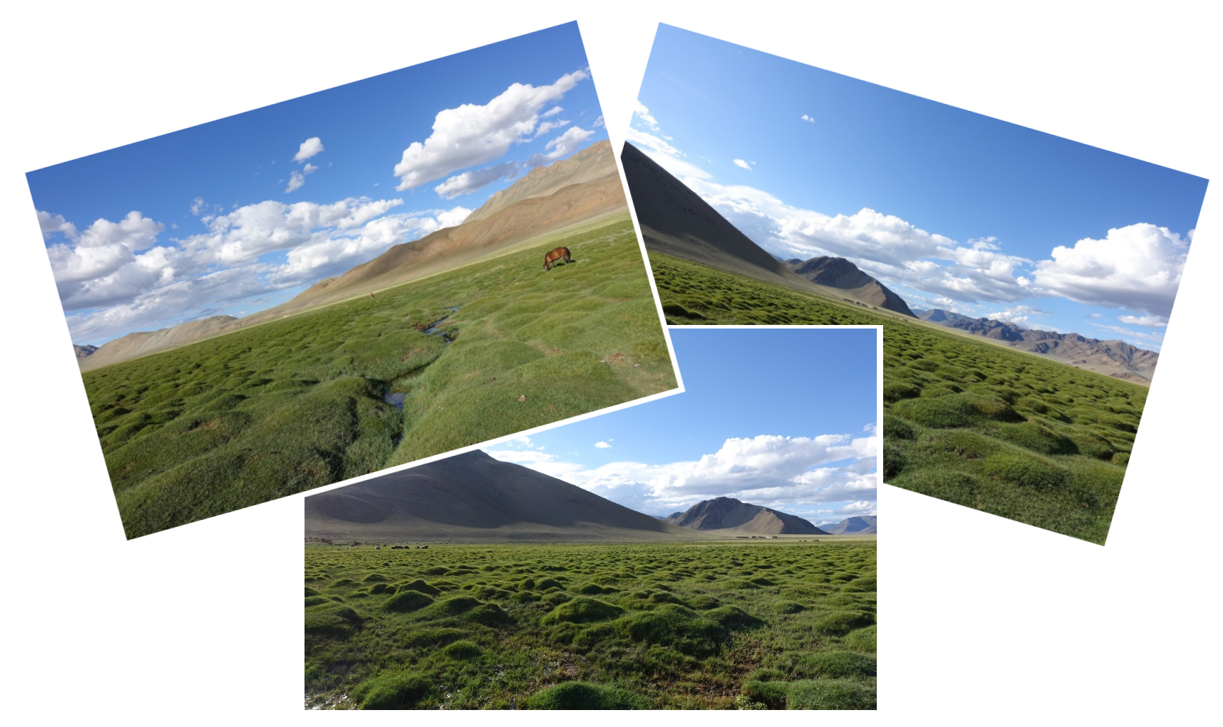

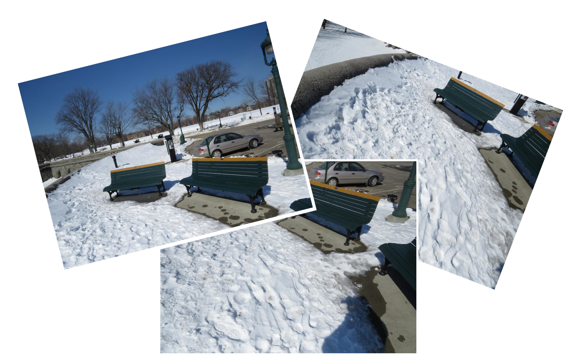
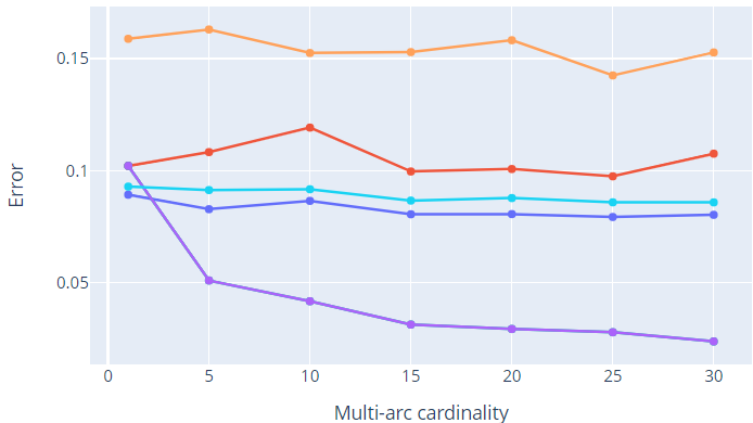
To decide the quality of a match the Lowe’s ratio-test is used with a threshold matching_threshold set to \(0.7\). Once the salient matches are selected, a homography is estimated from them only if a sufficient number of matches is present, i.e., if there are more than matches_th, set to \(30\). Regarding the RANSAC algorithm, the maximum number of iterations RANSACmaxIters is set to \(2000\). Also, the cardinality of the multi-arcs is represented by number_of_matches, set to \(10\). Furthermore, given the absence of ground truth to evaluate the correctness and goodness of the applied methods, we decided to implement a procedure that allows the creation of noisy images. In particular, the idea is to add some Gaussian noise to the points estimated by SIFT. Then, the methods are applied one by one and the resulting global homographies are compared with those obtained by applying simple-graph synchronization in a noise-free scenario, considered as ground truth. To compare the estimated labels \(x_i\) with the ground-truth ones \(x_{GT}\), the error is defined as the Frobenius norm of the deviation from the identity: \(\mathcal{E}_{i} = \| I_3 - (x_{GT} \; x_i^{-1})\|_{F} \quad \quad \forall i \in \mathcal{V}\) In this way, it is possible to understand the effectiveness of each method in dealing with noise data. The experiments have been conducted on different datasets 50 times to get a more robust estimate, changing the noise standard deviation and the multi-edge degree. It is important to notice that the multi-edge degree only influences Edge-Averaging stitching and Multi-graph stitching since they work on multi-graphs.
Let’s now analyze the results.
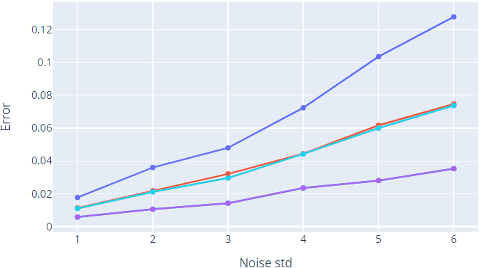
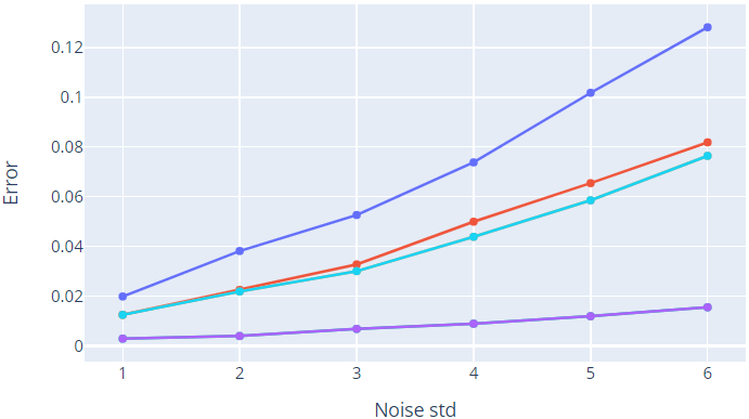
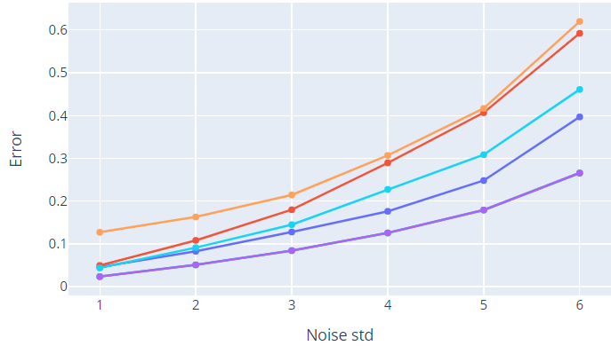
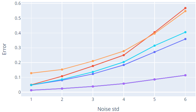


Basic stitching is the simplest, fastest and most intuitive method that we analysed. It can work even with acyclic graphs, however, given the fact that images are added one at a time to the mosaic, the error tends to accumulate. In fact, this approach does not exploit any global information but only the local one present in the two images that are being stitched.
Simple-graph stitching tries to overcome this problem by exploiting cycles present in the graph and distributing the error that is present on the single edges. In principle, this should allow producing better results than the previous method. However, we noticed that while on real data (noise-free scenario), the results produced by the two methods are almost identical from a qualitative point of view, those produced on synthetic data vary according to the dataset that is used.
We believe that this is due to the fact that Simple-graph stitching has a higher probability to encounter outlier edges since it takes into consideration all the edges present in the graph (while Basic stitching only considers a subset of them). Outlier edges are edges heavily affected by noise, that bring a negative contribution to the overall performance of the method. A more robust procedure should be taken into consideration in future works.
Multi-graph stitching (our first proposed approach) reaches the best results on all of the datasets. The key advantage over other methods is that it takes into consideration multi-arcs, thus outperforming methods based on simple graphs. Note that when considering the Multi-arc cardinality equal to one, the performance of Multi-graph stitching and Simple Graph stitching are the same (this is obvious since Multi-graph reduces to Simple-graph). Increasing the multi-arc cardinality reduces the error and results become better and better. This is due to the fact that having multiple measurements between the same pair of nodes (i.e., higher multi-arc cardinality) guarantees more robustness to noise.
Edge-Averaging stitching also exploit the information from the multi-edges, in a more naive way w.r.t. Multi-graph stitching. Surprisingly, in our results, the performance of the two methods is the same. Note that no theoretical guarantees are present in the case of Edge-Averaging stitching. Several experiments demonstrated that the average of the edges is still close to be in SL(3). This aspect should be better analysed in the future.
Regarding Multi-Patch stitching (the other proposed method), we observed that it performs worse than the others on some datasets in a noise-free scenario while it is always the worst when noise is added. Using its variant Multi-Patch Edge-Averaging stitching, performances seem to get better in many cases, being comparable to those provided by Basic stitching and Simple-graph stitching.
Given that Multi-Patch stitching solves synchronization problems on each patch locally, the solution obtained by synchronizing the patch graph is not guaranteed to be the global optimum since only a portion of the available global information is exploited. Thus, it is reasonable that its performances are worse than methods not based on patches. However, Multi-Patch Edge-Averaging stitching seems to reduce this effect.
Also in this case, there are no theoretical guarantees regarding the average over homographies, thus this could be a starting point for future analysis. Independently of the method that is used, the error increases when noise is bigger intuitively. Instead, fixing the noise and increasing the multi-edge degree allows to improve the results of methods based on multi-graphs following the theoretical expectations.
The obtained results show the effectiveness of MULTISYNC
- Investigating the relationship between the results obtained with Multi-Graph stitching and Edge-Averaging stitching.
- Investigating the relationship between the results obtained with Multi-patch stitching and Multi-patch Edge-Averaging stitching.
- Considering the introduction of multi-arcs in patch synchronization for partition mosaicing, using MULTISYNC for each cluster instead of the spectral solution.
- Collecting more challenging datasets to evaluate the performances of multi-graph based methods on real data introducing when possible a ground truth.
You can find the implementation in the linked repository.